Lacking Sample Data? Generate it
Why would you approximate a model from data generated by that same exact model?
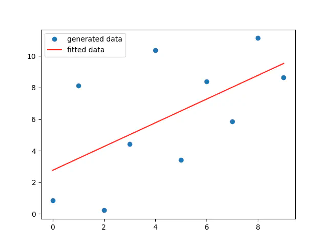 figure 1
Introduction
In case an author or a blogger tried to show how some data-science or machine-learning model works, Usually he/she brings a sample dataset, then apply the model on it. What if you wished to do your first hello-world test but have no sample data? In this post, I am going to show you how to generate such data. Surprisingly, the data shall be generated from the same model you are approximating!
Contents
- Introduction
- Just an Ordinary Line
- Introducing Noise, But Not a Random One
- Insights on Chosen Distribution
- Forget The Known Right Answer, Then Estimate it
- Our Behavior isn’t Purely Statistical
- Concrete Code
- Summary
Just an Ordinary Line
We shall use the linear model as an example. However, the procedure could be applied on nearly any other model. Basically, You assume the model’s parameters, in our linear model’s case, that would be both the intercept and slope. Then you compute couple of points via the model whose parameters are assumed. up to this point, the points shall strictly follow a straight line, as they are generated by a linear model.
Introducing Noise, But Not a Random One

In order to provide a more reliable test for our model, We shall introduce noise via the standard normal distribution. That is the core trick of the method. As you see in the upper graph, Its peak is exactly at 0, then it falls as we tend to either positive or negative side. That means, if we picked-up a number randomly, then the highest probability of that number is to be 0, and the more we tend towards the positive or negative x-values, the less chances of our randomly picked-up number to be equal to the corresponding x-value. The process we have just described is called sampling from a probability distribution.
So, how do we benefit from sampling the standard normal distribution in order to apply noise so that our generated data would not fall within a strict straight line? Basically, you just add the sampled number to the point generated by the linear model. You might wish to multiply the sampled number by some constant so that you gain a more significant noise.
Insights on Chosen Distribution
Note that the positive side of the standard normal distribution acts as a mirror to the negative side, So our chances are the same for sampling a positive or negative number. As a result, after adding the sampled number, the generated point would move either upper or below the line with equal chances. Check out the graph in the beginning of the page (figure 1) and see how this note applies to it.
Another worth to mention note is that the number of points close to the line are greater than the number of points faraway from the line, as shown in the same graph. That conforms with our illustration of standard normal distribution where the sample’s chances are greatest near the zero. If we expect more numbers to be near the zero, then certainly more points shall be near the line as the summation of low values diverges points minimally from the line.
Forget The Known Right Answer, Then Estimate it
After generating some points, you forget about the model’s assumed parameters, in our case, the intercept and slope. then you estimate the model’s parameters from these generated points.
Our Behavior isn’t Purely Statistical
We have just hand-crafted data by well-known statistical methods. In real-life, you wouldn’t have a prior knowledge of the data like that. In addition, Humans behavior does not seem to purely follow statistics in the same way an equation does. So, be cautious of your metrics while working on statistically generated data. Dealing with this data is alike printing hello world to test whether everything is okay before delving into actual work. By the way, I find it so curious to place a rigor discipline like mathematics within the paradigm of human behavior/emotions. I guess you know where to look now for these intriguing investigations.
Concrete Code
For completeness and your own convenience, I shall show a python code on linear regression. Place all the files in the same folder, run dataGen.py to generate data statistically, then run main.py to compute the rest of the procedure, as illustrated earlier.
iniGues.py
import numpy as np

# assumed parameters
x0 = np.array([1, 1])
mapFunc.py
# linear model
def linear(inp, x):
	return (inp*x[1])+x[0]
dataGen.py
# Generating Data Statistically

# 3rd-party libraries
import numpy as np
# local files
import mapFunc
import iniGues as inG

# number of generated points
N = 10
# generated-points storage
lines = []

# initializing an empty file on memory
f = open("data.txt", "w")

# generate N points, then store them temporarily in lines array
#	apply mapping function giving x-point and initial-guess array, then add a random number. finally, convert to strings before appending
for i in range(N):
	lines.append(str(i) + " " + str(mapFunc.linear(i, inG.x0) + (3*np.random.randn())) + "\n")

# write lines' strings on the file, each element as a line
f.writelines(lines)	# the last '\n' is unwittingly ignored

# frees memory from the file
f.close()
main.py
import numpy as np

import matplotlib.pyplot as plt
from scipy import stats

data = [
	[],
	[]
]

# read data from file
# ---------------------------------

# opens file in memory
f = open("data.txt","r")

# reads untill no more lines are available
while(1):
	line = f.readline()
	if (line == ""):
		break

	# split at space; last character, '\n', is unwittingly ignored
	line_split = line.split()

	# convert string to integer, then store each
	data[0].append(float(line_split[0]))
	data[1].append(float(line_split[1]))

# frees memory from the file
f.close()


# regression implementation
# ---------------------------------

# compute the linear regression
res = stats.linregress(data[0], data[1])

# store data computed by the linear model
resData = []
for i in range (len(data[0])):
	resData.append(res.intercept + (res.slope*data[0][i]))

# show results
# ---------------------------------

# show intercept, slope, .. etc
print(res)

# plot both the original and fitted models, colored blue and red, respectively
plt.plot(data[0], data[1], 'o', label='generated data')
plt.plot(data[0], resData, 'r', label='fitted data')
plt.legend()
plt.savefig('foo.png')
#plt.show()		alternatively, comment plt.savefig and comment out plt.show
Summary
Pick-up any model of your interest, and assume some parameters (end solution). Generate data by it but add noise by sampling from the standard normal distribution. Since the model is symmetric and probabillity chances falls as x-values tend either positively or negatively, The generated points are expected to equally diverge upper and below the exact point expected by the model before adding noise, and the generated points diverge is more likely to be minimal. Afterwards, The model’s parameters are estimated via the generated points. Precaution must be taken as real-life data usually do not strictly follow statistical characteristics. Finally, A supplementary code is provided on linear regression.